מבוא ל-Qiskit

במחברת זו נחקור כיצד ניתן לתכנת שערי קוונטים ומעגלי קוונטים עם Qiskit ואפילו כיצד ניתן להריץ אותם על סימולטורים ומחשבים קוונטיים אמיתיים באמצעות דפוסי Qiskit. בהמשך נציג דרכים שונות לקידוד מידע ונסיים עם דוגמת בונוס של טלפורטציה קוונטית.

לפני שמתחילים

עקוב אחר הוראות ההתקנה וההגדרה אם עדיין לא עשית זאת, כולל השלבים להגדרת שימוש ב-IBM Quantum™ Platform.

מומלץ להשתמש בסביבת הפיתוח Jupyter לאינטראקציה עם מחשבים קוונטיים. הקפד להתקין את תמיכת הוויזואליזציה הנוספת המומלצת ('qiskit[visualization]'). תצטרך גם את חבילת matplotlib עבור החלק השני של הדוגמה.

כדי ללמוד על מחשוב קוונטי בכלל, כנס לקורס יסודות המידע הקוונטי ב-IBM Quantum Learning

ייבוא

# Added by doQumentation — required packages for this notebook
!pip install -q matplotlib numpy qiskit qiskit-aer qiskit-ibm-runtime

# Import necessary modules for this notebook
import time
import qiskit

from qiskit import QuantumCircuit
from qiskit.quantum_info import Statevector
from qiskit.visualization import plot_bloch_multivector, plot_state_qsphere
from qiskit_aer import AerSimulator
from qiskit.quantum_info import SparsePauliOp
from qiskit.transpiler.preset_passmanagers import generate_preset_pass_manager
from qiskit_ibm_runtime import EstimatorV2 as Estimator
from qiskit_ibm_runtime import SamplerV2 as Sampler
from qiskit_ibm_runtime import QiskitRuntimeService
from qiskit.visualization import plot_histogram
print(qiskit.__version__)

2.3.1

כדי להריץ את מעגלי הקוונטים שלך על חומרה, עליך קודם להגדיר את החשבון שלך. ניתן לעשות זאת באופן הבא:

1. עבור אל פלטפורמת IBM Quantum® המשודרגת.
2. עבור לפינה הימנית העליונה (כפי שמוצג בתמונה לעיל), צור את אסימון ה-API שלך והעתק אותו למיקום מאובטח.
3. בתא הבא, החלף את deleteThisAndPasteYourAPIKeyHere במפתח ה-API שלך.
4. עבור לפינה השמאלית התחתונה (כפי שמוצג בתמונה לעיל) וצור את המופע שלך. הקפד לבחור בתוכנית הפתוחה.
5. לאחר יצירת המופע, העתק את קוד ה-CRN המשויך אליו. ייתכן שתצטרך לרענן כדי לראות את המופע.
6. בתא למטה, החלף את deleteThisAndPasteYourCRNHere בקוד ה-CRN שלך.

ראה מדריך זה לפרטים נוספים על הגדרת חשבון IBM Cloud® שלך.

⚠️ הערה: טפל במפתח ה-API שלך כפי שהיית מטפל בסיסמה מאובטחת. ראה את המדריך הגדרת Cloud לקבלת מידע נוסף על שימוש במפתח ה-API שלך בסביבות מאובטחות ובלתי מהימנות.

#your_api_key = "deleteThisAndPasteYourAPIKeyHere"
#your_crn = "deleteThisAndPasteYourCRNHere"

QiskitRuntimeService.save_account(
    channel="ibm_quantum_platform",
    token=your_api_key,
    instance=your_crn,
    overwrite=True
)

1. שערי קוונטים ומעגלי קוונטים

מעגלי קוונטים הם מודלים לחישוב קוונטי שבהם חישוב הוא רצף של שערי קוונטים. בוא נסתכל על כמה מהשערים הקוונטיים הפופולריים.

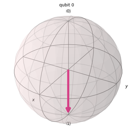
X Gate

X Gate שווה לסיבוב סביב ציר ה-X של כדור Bloch ב-$\pi$ רדיאנים. הוא ממפה $|0\rangle$ ל-$|1\rangle$ ו-$|1\rangle$ ל-$|0\rangle$. זהו המקבילה הקוונטית של שער ה-NOT למחשבים קלאסיים ולעיתים נקרא היפוך-סיבית.

$X = \begin{pmatrix} 0 & 1 \\ 1 & 0 \\ \end{pmatrix}$

# Let's apply an X-gate on a |0> qubit
qc = QuantumCircuit(1)
qc.x(0)
qc.draw(output='mpl')

# Let's see Bloch sphere visualization
sv = Statevector(qc)
plot_bloch_multivector(sv)

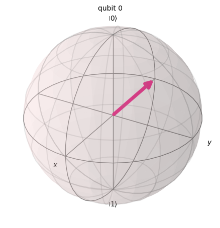
H Gate

H Gate מייצג סיבוב של $\pi$ סביב הציר שנמצא באמצע הציר $X$ ובין הציר $Z$. הוא ממפה את מצב הבסיס $|0\rangle$ ל-$\frac{|0\rangle + |1\rangle}{\sqrt{2}}$, מה שאומר שמדידה תהיה בעלת הסתברויות שוות להיות 1 או 0, ויוצר 'סופרפוזיציה' של מצבים. מצב זה נכתב גם כ-$|+\rangle$.

$H = \frac{1}{\sqrt{2}}\begin{pmatrix} 1 & 1 \\ 1 & -1 \\ \end{pmatrix}$

# Let's apply an H-gate on a |0> qubit
qc = QuantumCircuit(1)
qc.x(0)
qc.h(0)
qc.draw(output='mpl')

# Let's see Bloch sphere visualization
sv = Statevector(qc)
plot_bloch_multivector(sv)

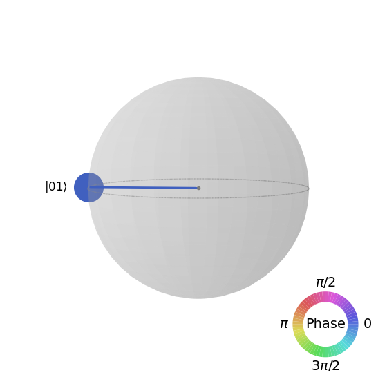
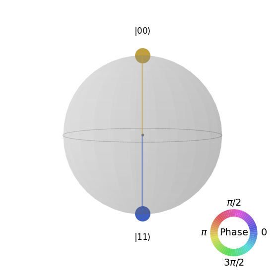
CX Gate (CNOT Gate)

שער ה-NOT המבוקר (או CNOT או CX) פועל על שני Qubitים. הוא מבצע את פעולת ה-NOT (שווה ערך להחלת X Gate) על ה-Qubit השני רק כאשר ה-Qubit הראשון הוא $|1\rangle$ ואחרת משאיר אותו ללא שינוי. הערה: Qiskit ממספר את הביטים במחרוזת מימין לשמאל.

$CX = \begin{pmatrix} 1 & 0 & 0 & 0\\ 0 & 1 & 0 & 0\\ 0 & 0 & 0 & 1\\ 0 & 0 & 1 & 0\\ \end{pmatrix}$

# Let's apply a CX-gate on |11>
qc = QuantumCircuit(2)
qc.x(0)
qc.x(1)
qc.cx(0,1)
qc.draw(output='mpl')

sv=Statevector(qc)
plot_state_qsphere(sv)

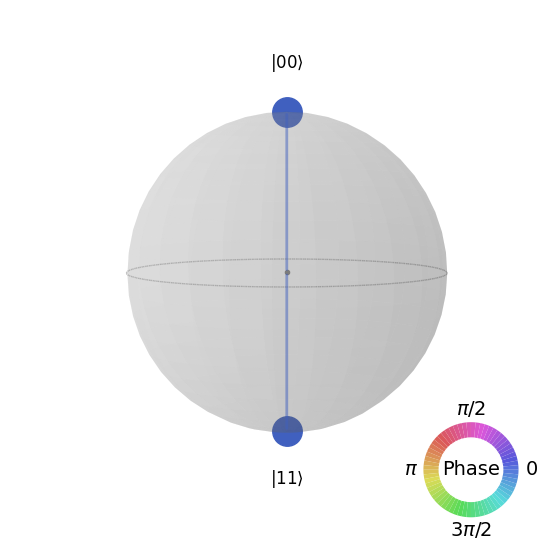
צור את מצב Bell הראשון

$|\phi^+ \rangle = \frac{1}{\sqrt 2}(|00 \rangle + |11 \rangle)$

# Create a Bell state circuit

qc = QuantumCircuit(2)
qc.h(0)
qc.cx(0,1)

# Draw the circuit
qc.draw("mpl")

# Plot the state using q-sphere visualization
sv = Statevector(qc)
plot_state_qsphere(sv)
# q-sphere is useful for visualizing states when Bloch sphere fails to

צור את מצב Bell השני

$|\phi^- \rangle = \frac{1}{\sqrt 2}(|00 \rangle - |11 \rangle)$

# Create a circuit with the second Bell state

qc = QuantumCircuit(2)
qc.x(0)
qc.h(0)
qc.cx(0,1)

qc.draw("mpl")

ההסבר הוא:

$$H|1\rangle=\frac{1}{\sqrt{2} }(|0\rangle-|1\rangle) = |-\rangle$$

# Get the statevector of the circuit
sv = Statevector(qc)

# Plot the state using qsphere visualization
plot_state_qsphere(sv)

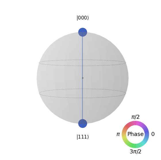
צור את מצב GHZ בן 3 Qubitים

$|GHZ \rangle = \frac{1}{\sqrt 2}(|000 \rangle + |111 \rangle)$

# Create a circuit with 3-qubit GHZ state

qc= QuantumCircuit(3)
qc.h(0)
qc.cx(0,1)
qc.cx(0,2)

qc.draw("mpl")

# Get the statevector of the circuit
sv = Statevector(qc)

# Plot the state using qsphere visualization
plot_state_qsphere(sv)

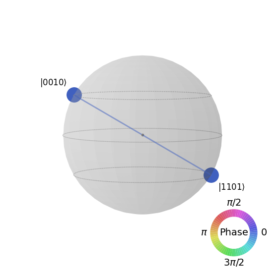
צור את מצב לוגו Qiskit

$|Qiskit \rangle = \frac{1}{\sqrt 2}(|0010 \rangle + |1101 \rangle)$

# Create a circuit with the Qiskit logo state

qc = QuantumCircuit(4)
qc.h(0)
qc.cx(0,1)
qc.cx(0,2)
qc.cx(0,3)
qc.x(1)

# Draw the circuit
qc.draw("mpl")

# Get the statevector of the circuit
sv = Statevector(qc)

# Plot the state using qsphere visualization
plot_state_qsphere(sv)

2. צור והרץ תוכנית קוונטית פשוטה

ארבעת השלבים לכתיבת תוכנית קוונטית באמצעות דפוסי Qiskit הם:

1. ממפים את הבעיה לפורמט מקורי קוונטי.

2. מייעלים את ה-Circuit והאופרטורים.

3. מבצעים את הפעולה באמצעות פונקציית Estimator/Sampler קוונטית פרימיטיבית.

4. מנתחים את התוצאות.

2.1 מיפוי הבעיה לפורמט קוונטי-נייטיב

בתוכנית קוונטית, Circuit קוונטיים הם הפורמט הנייטיב לייצוג הוראות קוונטיות, ו-אופרטורים מייצגים את האובייקטים הנמדדים. כשיוצרים Circuit, בדרך כלל יוצרים אובייקט QuantumCircuit חדש ואז מוסיפים אליו הוראות ברצף.

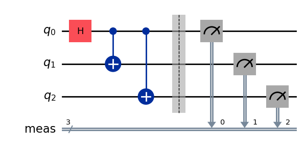
תא הקוד הבא יוצר Circuit שמייצר את מצב GHZ — מצב שבו שלושה Qubit שזורים לחלוטין אחד עם השני.

ה-Qiskit SDK משתמש במספור סיביות LSb 0, שבו הספרה ה-$n$ בעלת הערך $1 \ll n$ או $2^n$. לפרטים נוספים, ראו את הנושא Bit-ordering in the Qiskit SDK.

# Create a GHZ state circuit

qc = QuantumCircuit(3)
qc.h(0)
qc.cx(0,1)
qc.cx(0,2)
# Draw the circuit
qc.draw("mpl")

ראו את QuantumCircuit בתיעוד לכל הפעולות הזמינות.

כשיוצרים Circuit קוונטיים, צריך גם לשקול איזה סוג של נתונים רוצים לקבל בחזרה אחרי הרצה. Qiskit מציע שתי דרכים להחזרת נתונים: אפשר לקבל התפלגות הסתברות עבור קבוצת Qubit שבוחרים למדוד, או לקבל את ערך הציפייה של אובייקט נמדד. הכינו את העומס שלכם למדוד את ה-Circuit באחת משתי הדרכים האלה באמצעות primitives של Qiskit (מוסבר בפירוט בשלב 3).

הדוגמה הזו מודדת ערכי ציפייה באמצעות מודול המשנה qiskit.quantum_info, שמצוין באמצעות אופרטורים (אובייקטים מתמטיים המשמשים לייצוג פעולה או תהליך שמשנים מצב קוונטי). תא הקוד הבא יוצר שישה אופרטורי פאולי של שלושה Qubit: ZZZ, ZZX, ZII, XXI, ZZI ו-III.

# Set up six different observables.

observables_labels = ["ZZZ", "ZZX", "ZII", "XXI", "ZZI", "III"]

observables = [SparsePauliOp(label) for label in observables_labels]
print(observables)

[SparsePauliOp(['ZZZ'],
              coeffs=[1.+0.j]), SparsePauliOp(['ZZX'],
              coeffs=[1.+0.j]), SparsePauliOp(['ZII'],
              coeffs=[1.+0.j]), SparsePauliOp(['XXI'],
              coeffs=[1.+0.j]), SparsePauliOp(['ZZI'],
              coeffs=[1.+0.j]), SparsePauliOp(['III'],
              coeffs=[1.+0.j])]

כאן, משהו כמו האופרטור ZZI הוא קיצור למכפלה הטנזורית $Z\otimes Z\otimes I$, כלומר מדידת Z על Qubit 2 ו-Z על Qubit 1 יחד, ולקבל מידע על הקורלציה בין Qubit 2 ל-Qubit 1. ערכי ציפייה כאלה נכתבים בדרך כלל גם כ-$\langle Z_2 Z_1 \rangle$.

אם המצב שאנחנו מתבוננים בו הוא מצב GHZ של שלושה Qubit, אז המדידה של $\langle Z_2 Z_1 \rangle$ אמורה להיות 1.

2.2 אופטימיזציה של ה-Circuit והאופרטורים

כשמריצים Circuit על מכשיר, חשוב לאמטב את קבוצת ההוראות שה-Circuit מכיל ולמזער את העומק הכולל (בגדול, מספר ההוראות) של ה-Circuit. הדבר מבטיח שתקבלו את התוצאות הטובות ביותר האפשריות על ידי הפחתת השפעות השגיאה והרעש. בנוסף, הוראות ה-Circuit חייבות לעמוד ב-Instruction Set Architecture (ISA) של ה-Backend ולקחת בחשבון את Gate הבסיסיים וקישוריות ה-Qubit של המכשיר.

הקוד הבא יוצר מופע של מכשיר אמיתי לשליחת עבודה אליו, ומתמיר את ה-Circuit והאופרטורים כך שיתאימו ל-ISA של אותו Backend. אם לא שמרתם את האישורים שלכם קודם לכן, עקבו אחר ההוראות כאן לאימות עם ה-API token שלכם.

# Choose a real backend
service = QiskitRuntimeService(channel='ibm_quantum_platform',)
backend = service.least_busy(min_num_qubits=156)
# print backend details
print(
    f"Name: {backend.name}\n"
    f"Version: {backend.backend_version}\n"
    f"No. of qubits: {backend.num_qubits}\n"
    f"Processor type: {backend.processor_type}\n"
)

Name: ibm_marrakesh
Version: 1.0.21
No. of qubits: 156
Processor type: {'family': 'Heron', 'revision': '2'}

# option to use the AerSimulator instead of a real quantum device
seed_sim=42
backend=AerSimulator.from_backend(backend,seed_simulator=seed_sim)

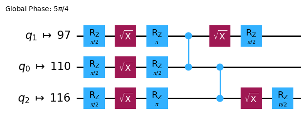
בצעו Transpile על ה-Circuit ל-ISA Circuit

# Convert to an ISA circuit and layout-mapped observables.

pm = generate_preset_pass_manager(backend=backend, optimization_level=2)
isa_circuit = pm.run(qc) 

isa_circuit.draw("mpl", idle_wires=False)

mapped_observables = [
    observable.apply_layout(isa_circuit.layout) for observable in observables
]
print(mapped_observables)

[SparsePauliOp(['IIIIIIIIIIIIIIIIZIIIIIZIIIIIIIIIIIIZIIIIIIIIIIIIIIIIIIIIIIIIIIIIIIIIIIIIIIIIIIIIIIIIIIIIIIIIIIIIIIIIIIIIIIIIIIIIIIIIIIIIIIIIIIIIIIIII'],
              coeffs=[1.+0.j]), SparsePauliOp(['IIIIIIIIIIIIIIIIZIIIIIXIIIIIIIIIIIIZIIIIIIIIIIIIIIIIIIIIIIIIIIIIIIIIIIIIIIIIIIIIIIIIIIIIIIIIIIIIIIIIIIIIIIIIIIIIIIIIIIIIIIIIIIIIIIIII'],
              coeffs=[1.+0.j]), SparsePauliOp(['IIIIIIIIIIIIIIIIZIIIIIIIIIIIIIIIIIIIIIIIIIIIIIIIIIIIIIIIIIIIIIIIIIIIIIIIIIIIIIIIIIIIIIIIIIIIIIIIIIIIIIIIIIIIIIIIIIIIIIIIIIIIIIIIIIIII'],
              coeffs=[1.+0.j]), SparsePauliOp(['IIIIIIIIIIIIIIIIXIIIIIIIIIIIIIIIIIIXIIIIIIIIIIIIIIIIIIIIIIIIIIIIIIIIIIIIIIIIIIIIIIIIIIIIIIIIIIIIIIIIIIIIIIIIIIIIIIIIIIIIIIIIIIIIIIIII'],
              coeffs=[1.+0.j]), SparsePauliOp(['IIIIIIIIIIIIIIIIZIIIIIIIIIIIIIIIIIIZIIIIIIIIIIIIIIIIIIIIIIIIIIIIIIIIIIIIIIIIIIIIIIIIIIIIIIIIIIIIIIIIIIIIIIIIIIIIIIIIIIIIIIIIIIIIIIIII'],
              coeffs=[1.+0.j]), SparsePauliOp(['IIIIIIIIIIIIIIIIIIIIIIIIIIIIIIIIIIIIIIIIIIIIIIIIIIIIIIIIIIIIIIIIIIIIIIIIIIIIIIIIIIIIIIIIIIIIIIIIIIIIIIIIIIIIIIIIIIIIIIIIIIIIIIIIIIIII'],
              coeffs=[1.+0.j])]

2.3 הרצה באמצעות ה-primitives הקוונטיים

מחשבים קוונטיים יכולים לייצר תוצאות אקראיות, אז בדרך כלל אוספים דגימה מהפלטים על ידי הרצת ה-Circuit פעמים רבות. אפשר לאמוד את ערכו של האובייקט הנמדד באמצעות המחלקה Estimator. ה-Estimator הוא אחד משני primitives; השני הוא Sampler, שניתן להשתמש בו כדי לקבל נתונים ממחשב קוונטי. לאובייקטים האלה יש מתודת run() שמריצה את ה-Circuit, האופרטורים והפרמטרים הנבחרים (אם רלוונטי), תוך שימוש ב-primitive unified bloc (PUB). כשמריצים קוד זה על חומרת קוונטום אמיתית, כדאי להשתמש בטכניקות לצמצום ומיתון שגיאות כדי להפחית את הרעש הפנימי של המחשב הקוונטי.

# Construct the Estimator instance.
estimator = Estimator(mode=backend)
estimator.options.resilience_level = 1
estimator.options.default_shots = 5000

שלחו עבודה באמצעות ה-Estimator primitive.

# One pub, with one circuit to run against six different observables.
job = estimator.run([(isa_circuit, mapped_observables)]) 

# Use the job ID to retrieve your job data later
print(f">>> Job ID: {job.job_id()}")

>>> Job ID: 97ecd036-1767-49b0-a1dc-c71638c3c3c4

/Users/jma/miniconda3/envs/3122/lib/python3.12/site-packages/qiskit_ibm_runtime/fake_provider/local_service.py:187: UserWarning: The resilience_level option has no effect in local testing mode.
  warnings.warn("The resilience_level option has no effect in local testing mode.")

אחרי שעבודה נשלחה, אפשר לחכות עד שתסתיים בתוך מופע ה-Python הנוכחי, או להשתמש ב-job_id כדי לאחזר את הנתונים מאוחר יותר. (ראו את הקטע על אחזור עבודות לפרטים.)

אחרי שהעבודה מסתיימת, בחנו את הפלט שלה דרך המאפיין result() של העבודה.

# This is the result of the entire submission.  You submitted one Pub,
# so this contains one inner result (and some metadata of its own).
job_result = job.result()

# This is the result from our single pub, which had six observables,
# so contains information on all six.
pub_result = job.result()[0]

עכשיו אפשר גם להריץ את ה-Circuit באמצעות ה-Sampler primitive

# We include the measurements in the circuit
qc.measure_all()
sampler = Sampler(mode=backend)

qc.draw(output="mpl")

שלחו עבודה באמצעות ה-Sampler primitive.

job_sampler = sampler.run(pm.run([qc]))

# Use the job ID to retrieve your job data later
print(f">>> Job ID: {job_sampler.job_id()}")
# Get the results
results_sampler = job_sampler.result()

>>> Job ID: a6ee4d2f-c80d-4a86-9a76-e4b1a74502e7

2.4 ניתוח התוצאות

שלב הניתוח הוא בדרך כלל המקום שבו אפשר לעבד מחדש את התוצאות, למשל באמצעות הפחתת שגיאות מדידה או אקסטרפולציה של אפס רעש (ZNE). אפשר להזין את התוצאות האלה לתהליך עבודה אחר לניתוח נוסף, או להכין גרף של הערכים והנתונים המרכזיים. בדרך כלל, השלב הזה ספציפי לבעיה שלך. בדוגמה הזו, נשרטט כל אחד מערכי הציפייה שנמדדו עבור ה-Circuit שלנו.

ערכי הציפייה וסטיות התקן עבור האובזרבלות שציינת ל-Estimator נגישים דרך המאפיינים PubResult.data.evs ו-PubResult.data.stds של תוצאת העבודה. כדי לקבל את התוצאות מה-Sampler, השתמש בפונקציה PubResult.data.meas.get_counts(), שתחזיר dict של מדידות בצורת מחרוזות ביטים כמפתחות וספירות כערכים המתאימים. למידע נוסף, ראה Get started with Sampler.

# Plot the result
from matplotlib import pyplot as plt
values = pub_result.data.evs
errors = pub_result.data.stds
# plotting graph
# Plotting with error bars
plt.errorbar(observables_labels, values, yerr=errors, fmt='-o', capsize=5)
plt.xlabel("Observables")
plt.ylabel("Values")
plt.title("Plot of Observables vs Values with Error Bars")
plt.grid(True)
plt.tight_layout()
plt.show()

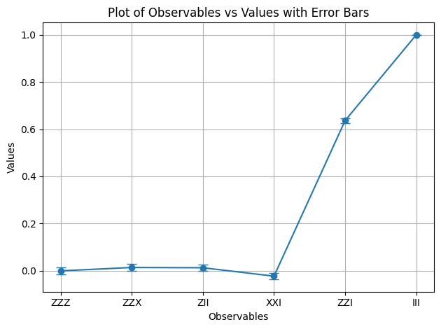
אנחנו רואים שלאובזרבלות $ZZI$ ו-$III$ יש ערך ציפייה של 1, מכיוון ש-$ZZI$ מכניס שני סימני מינוס שמתבטלים, ו-$III$ פועל כזהות ומשאיר את מצב ה-GHZ ללא שינוי. לשאר האובזרבלות יש ערך ציפייה של 0, מכיוון שאופרטורי ה-$Z$ שלהן מכניסים מספר אי-זוגי של סימני מינוס, או שאופרטורי ה-$X$ הופכים מספר של Qubitים שהופך את המצבים החופפים לאורתוגונליים.

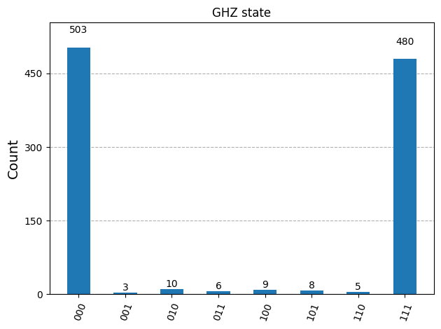
עכשיו נשרטט את התוצאות עבור ה-Sampler

counts_list = results_sampler[0].data.meas.get_counts()
print(counts_list)
print(f"Outcomes : {counts_list}")
display(plot_histogram(counts_list, title="GHZ state"))

{'111': 480, '000': 503, '101': 8, '100': 9, '001': 3, '011': 6, '010': 10, '110': 5}
Outcomes : {'111': 480, '000': 503, '101': 8, '100': 9, '001': 3, '011': 6, '010': 10, '110': 5}

2.5 הרחבה למספרים גדולים של Qubitים

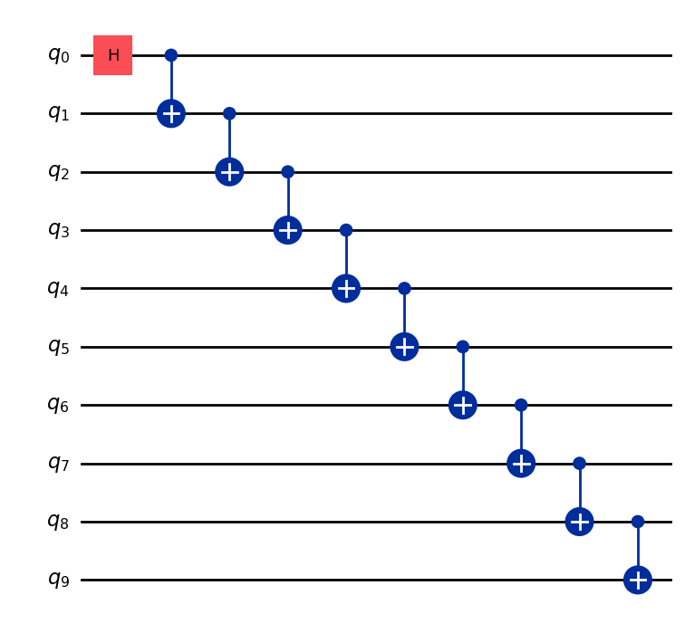
בחישוב קוונטי, עבודה בקנה מידה של שירות (utility-scale) היא קריטית להתקדמות בתחום. עבודה כזו דורשת ביצוע חישובים בקנה מידה גדול הרבה יותר — עם Circuitים שעשויים להשתמש ביותר מ-100 Qubitים וביותר מ-1000 Gateים. הדוגמה הזו עושה צעד קטן לכיוון הזה ומרחיבה את בעיית ה-GHZ ל-$n=10$ Qubitים. היא משתמשת בתהליך העבודה של Qiskit patterns ומסיימת במדידת ערך הציפייה $\langle Z_0 Z_i \rangle$.

שלב 1. מיפוי הבעיה

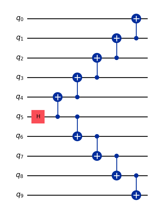
כתוב פונקציה שמחזירה QuantumCircuit שמכין מצב GHZ בגודל $n$ Qubitים (בעצם מצב Bell מורחב), ואז השתמש בפונקציה הזו להכנת מצב GHZ של 10 Qubitים ואסוף את האובזרבלות שיש למדוד.

def get_qc_for_n_qubit_GHZ_state(n: int) -> QuantumCircuit:

    qc = QuantumCircuit(n) 
    qc.h(0)
    for i in range(n-1):
        qc.cx(i, i+1)
    return qc
n = 10
qc_n_GHZ = get_qc_for_n_qubit_GHZ_state(n)
qc_n_GHZ.draw("mpl")

לאחר מכן, מפה לאופרטורים שמעניינים אותנו. הדוגמה הזו משתמשת באופרטורי ZZ בין Qubitים כדי לבחון את ההתנהגות ככל שהם מתרחקים זה מזה. ערכי ציפייה פחות מדויקים (פגומים) בין Qubitים מרוחקים יגלו את רמת הרעש הקיימת.

# ZZII...II, ZIZI...II, ... , ZIII...IZ
operator_strings = [
    "Z" + i * "I" + "Z" + "I" * (n-i-2) for i in range(n-1) 
]
print(operator_strings)
print(len(operator_strings))

operators = [SparsePauliOp(operator) for operator in operator_strings]

['ZZIIIIIIII', 'ZIZIIIIIII', 'ZIIZIIIIII', 'ZIIIZIIIII', 'ZIIIIZIIII', 'ZIIIIIZIII', 'ZIIIIIIZII', 'ZIIIIIIIZI', 'ZIIIIIIIIZ']
9

שלב 2. אופטימיזציה של הבעיה לביצוע על Backend קוונטי

המר את ה-Circuit והאובזרבלות כדי שיתאימו ל-ISA של ה-Backend.

# Convert to an ISA circuit and layout-mapped observables.
pm = generate_preset_pass_manager(backend=backend, optimization_level=2)
isa_circuit = pm.run(qc_n_GHZ) 
isa_operators_list = [operator.apply_layout(isa_circuit.layout) for operator in operators]

שלב 3. ביצוע על Backend

שלח את העבודה, ואם אתה מריץ אותה על חומרה, הפעל דיכוי שגיאות באמצעות טכניקה להפחתת שגיאות הנקראת dynamical decoupling. רמת החוסן (resilience level) מציינת כמה חוסן לבנות נגד שגיאות. רמות גבוהות יותר מייצרות תוצאות מדויקות יותר, על חשבון זמן עיבוד ארוך יותר. להסבר נוסף על האפשרויות שמוגדרות בקוד הבא, ראה Configure error mitigation for Qiskit Runtime.

# Submit the circuit to Estimator
job = estimator.run([(isa_circuit, isa_operators_list)])
job_id = job.job_id()

/Users/jma/miniconda3/envs/3122/lib/python3.12/site-packages/qiskit_ibm_runtime/fake_provider/local_service.py:187: UserWarning: The resilience_level option has no effect in local testing mode.
  warnings.warn("The resilience_level option has no effect in local testing mode.")

שלב 4. עיבוד מחדש של התוצאות

כדי להבין טוב יותר את ההתנהגות של מצבים קוונטיים שזורים על חומרה אמיתית, אנחנו מנתחים את המתאמים הזוגיים בין Qubitים בבסיס Z. ספציפית, אנחנו מסתכלים על ערכי הציפייה ⟨Z₀Zᵢ⟩, שמודדים כמה חזק Qubit 0 מתואם עם כל Qubit אחר i. בפרט, נשרטט:

$$\langle Z_i Z_0 \rangle / \langle Z_1 Z_0 \rangle$$

אילו ערכים של $\langle Z_i Z_0 \rangle / \langle Z_1 Z_0 \rangle$ אתה מצפה לראות בגרף?

אפשרויות:

א) יורד ככל שמגדילים את $i$

ב) קבוע ב-1

ג) סטיות קטנות סביב 1

ד) לסירוגין 1 ו-0 עבור ערכים אי-זוגיים וזוגיים של $i$

data = list(range(1, len(operators) + 1))  # Distance between the Z operators
result = job.result()[0]
values = result.data.evs  # Expectation value at each Z operator.
values = [
    v / values[0] for v in values
]  # Normalize the expectation values to evaluate how they decay with distance.

plt.plot(data, values, marker="o", label=f"{n}-qubit GHZ state")
plt.xlabel("Distance between qubits $i$")
plt.ylabel(r"$\langle Z_i Z_0 \rangle / \langle Z_1 Z_0 \rangle $")
plt.legend()
plt.show()

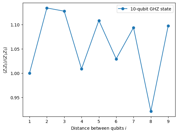
בגרף הזה אנחנו שמים לב ש-$\langle Z_0 Z_i \rangle$ מתנדנד סביב הערך 1, למרות שבסימולציה אידיאלית כל $\langle Z_0 Z_i \rangle$ אמורים להיות 1.

כפי שאפשר לראות, התוצאות של ניסויים עם 10 Qubitים טובות אבל עדיין יש בהן כמה שגיאות. אחת הדרכים לשפר את התוצאות היא לממש את מצב ה-GHZ בצורה יעילה יותר.

בדרך כלל מממשים מצב GHZ עם רצף של שערי CNOT בצורת מדרגות. אך אפשר לממש את מצב ה-GHZ בצורה יעילה יותר, ולהפחית את עומק ה-2-Qubit מ-n ל-n/2 או פחות.

מדד חשוב לבדיקת כמה מדויקות יהיו התוצאות, או כמה מעט רעש יהיה ל-Circuit, הוא עומק Gate של 2-Qubit. הסיבה לכך היא שקצבי השגיאה של Gateים של 2-Qubit (פי ~10 גבוהים יותר מ-Gateים של Qubit יחיד) שולטים בשגיאות של ה-Circuit כולו. השתמש בקוד הבא כדי לקבל את עומק ה-Gate של 2-Qubit של Circuit.

qc.depth(lambda x: x.operation.num_qubits == 2)

def better_ghz(n):
    "fan out"
    s = int(n / 2)
    qc = QuantumCircuit(n)
    qc.h(s)
    for m in range(s, 0, -1):
        qc.cx(m, m - 1)
        if not (n % 2 == 0 and m == s): 
            qc.cx(n - m - 1, n - m)
    return qc

better_ghz(n).draw("mpl")

# Check 2-qubit gate depth before transpilation
qc_better_ghz = better_ghz(n)
qc_better_ghz.depth(lambda x: x.operation.num_qubits == 2)

5

דבר מעניין לציין כאן הוא שהצלחנו להפחית את העומק הקוונטי של ה-Circuit שאנחנו רוצים להריץ, פשוט על ידי חשיבה חכמה ומציאת דרך שונה לתכנת אותו. אולם, יהיו מצבים ואלגוריתמים שבהם לא נוכל להסתמך על הטריקים החכמים האלה. כאן הTranspiler שימושי — הוא עוזר לנו לאופטימיזציה של כל ההיבטים האלה ביעילות, כך שאנחנו לא צריכים לדאוג יותר מדי לגביהם.

3. קידוד מידע

3.1 קידוד אמפליטודה

עכשיו שראינו איך לבנות מעגלים קוונטיים, מעניין לחקור איך אפשר לקדד מידע קלאסי לתוך מצבים קוונטיים. שיטה עוצמתית אחת היא קידוד אמפליטודה, שבו האמפליטודות של מצב קוונטי מייצגות את הרכיבים של וקטור קלאסי.

בוא נבחן דוגמה פשוטה. נניח שאנחנו רוצים לקדד את הוקטור הקלאסי

$$\vec{x} = \begin{bmatrix} x_0 \\ x_1 \\ x_2 \\ x_3 \end{bmatrix}$$

לתוך מצב קוונטי של שני Qubit. המטרה היא להכין את המצב הקוונטי:

$$\ket{\psi} = x_0\ket{00} + x_1\ket{01} + x_2\ket{10} + x_3\ket{11}$$

כאשר $x_0, x_1, x_2, x_3 \in \mathbb{R}$ (או $\mathbb{C}$) והוקטור מנורמל כך ש:

$$|x_0|^2 + |x_1|^2 + |x_2|^2 + |x_3|^2 = 1$$

עכשיו נבחן את הדוגמה הספציפית: $\vec{x} = [0.8924, 0.3696, 0.2391, 0.0990]$

אז המצב הקוונטי המתאים הוא:

$$\begin{aligned} \ket{\psi} &= 0.8924\,\ket{00} + 0.3696\,\ket{01} + 0.2391\,\ket{10} + 0.0990\,\ket{11} \end{aligned}$$

אפשר להכין מצב זה באמצעות שילוב של Gate-ים של סיבוב $R_y$ בזוויות $\pi/6$ ו-$\pi/4$ עבור Qubit 0 ו-1 בהתאמה

from qiskit import QuantumCircuit
from qiskit_aer import AerSimulator
import numpy as np

qc = QuantumCircuit(2)

qc.ry(np.pi / 6, 0)
qc.ry(np.pi / 4, 1)

simulator = AerSimulator()
qc.save_statevector()
result = simulator.run(qc).result()
statevector = result.get_statevector()

print("Statevector:", statevector)
qc.draw(output="mpl")

Statevector: Statevector([0.8923991 +0.j, 0.23911762+0.j, 0.36964381+0.j,
             0.09904576+0.j],
            dims=(2, 2))

from qiskit.quantum_info import Statevector

# Define our vector
v = np.array([0.8924,  0.3696, 0.2391, 0.0990]) 
v = v/np.linalg.norm(v)
# Create a statevector from the vector
state = Statevector(v)

# Initialize a quantum circuit with 2 qubits
qc = QuantumCircuit(2)
qc.initialize(state.data, [0, 1])

# Optional: simulate the state
print("Statevector:", state)

# Visualize the circuit
qc.decompose().decompose().decompose().decompose().decompose().draw("mpl")

Statevector: Statevector([0.89242154+0.j, 0.36960892+0.j, 0.23910577+0.j,
             0.09900239+0.j],
            dims=(2, 2))

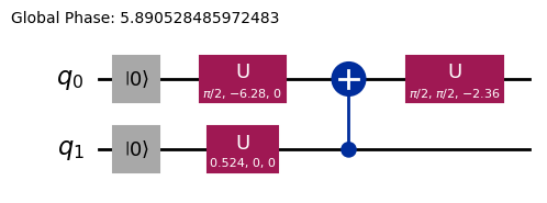
כך ראינו איך לקדד מידע באמצעות Gate-ים של סיבוב.

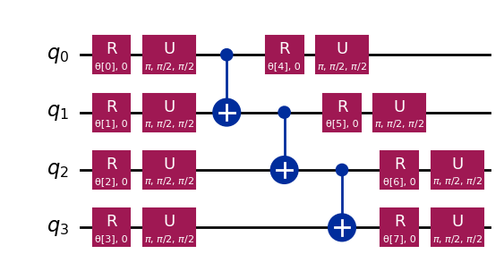
3.2 קידוד זווית ומעגלים פרמטריים

דרך מעניינת במיוחד לקדד מידע למחשב קוונטי היא לתכנן Circuit קוונטי שמכיל כמה זוויות סיבוב $\vec{\theta}$ או פרמטרים שניתן לכוונן כדי לייצג משפחה של פונקציות $f(\vec{\theta})$. בוא נבחן לדוגמה את ה-Circuit הקוונטי הפרמטרי הבא:

from qiskit import QuantumCircuit
from qiskit.circuit import Parameter

# Define a symbolic parameter
theta = Parameter("θ")

qc = QuantumCircuit(2)
# We applied a parametrized RX gate
qc.rx(theta, 0)
qc.cx(0, 1)
qc.draw("mpl")

מבחינה מתמטית, אפשר לנתח מהי משפחת הפונקציות שאפשר לייצג עם ה-Circuit הזה:

$$\text{CNOT}_{01} \, R_x^{\{0\}}(\theta) |00\rangle = \text{CNOT}_{01} \left( \cos(\theta/2)\ket{00} - i\sin(\theta/2)\ket{10} \right) = \cos(\theta/2)\ket{00} - i\sin(\theta/2)\ket{11}$$

די ברור שמספר המצבים שאפשר לייצג עם ה-Circuit הקוונטי הזה מוגבל, כי לא ניתן לייצג מצבים כמו $\ket{10}$ או $\ket{01}$ למשל. עם זאת, משפחת המצבים שאפשר לייצג מתרחבת כשמוסיפים סיבובים נוספים במקומות המתאימים:

from qiskit import QuantumCircuit
from qiskit.circuit import Parameter

# Define a symbolic parameter
theta1 = Parameter("θ1")
theta2 = Parameter("θ2")

qc = QuantumCircuit(2)
qc.rx(theta1, 0)
qc.rx(theta2, 1)
qc.cx(0, 1)
qc.draw("mpl")

במקרה זה, המצבים הקוונטיים שנייצג הם:

\begin{align*} \text{CNOT}_{01} \, R_x^{\{1}}(\theta_2) R_x^{\{0}}(\theta_1) \ket{00} &= \text{CNOT}_{01} \, R_x^{\{1}}(\theta_2)\left( \cos(\theta_1/2)\ket{00} - i\sin(\theta_1/2)\ket{10} \right) \\ &= \text{CNOT}_{01}\left( \cos(\theta_1/2)\cos(\theta_2/2)\ket{00} - i\cos(\theta_1/2)\sin(\theta_2/2)\ket{01} \right. \\ &\quad \left. - i\sin(\theta_1/2)\cos(\theta_2/2)\ket{10} + \sin(\theta_1/2)\sin(\theta_2/2)\ket{11} \right) \\ &= \cos(\theta_1/2)\cos(\theta_2/2)\ket{00} - i\cos(\theta_1/2)\sin(\theta_2/2)\ket{01} \\ &\quad + \sin(\theta_1/2)\sin(\theta_2/2)\ket{10} - i\sin(\theta_1/2)\cos(\theta_2/2)\ket{11} \end{align*}

אפשר לראות שה-Circuit הזה מייצר משפחה רחבה יותר של מצבים קוונטיים בהשוואה לקודמו. בפרט, עכשיו הוא יכול לייצר מצבים עם אמפליטודות שאינן אפס עבור $\ket{01}$ או $\ket{10}$ שלא היו אפשריים עם ה-Circuit שלמעלה. עם זאת, ה-Circuit הזה עדיין אינו מייצר מצבים קוונטיים כלליים, אם כי הוא עשוי להיות בעל מספיק ביטוי לתכנן Circuit-ים עם גמישות מסוימת לייצוג פונקציות מסוימות. באופן כללי, ככל שמוסיפים פרמטרים עצמאיים (זוויות) יותר, כך ל-Circuit יש יותר ביטויים לקרב מצבים קוונטיים שרירותיים.

Ansatzes וספריית ה-Circuit

סוג זה של Circuit קוונטי פרמטרי יכול לשמש לבניית Ansatzes, מצבים קוונטיים ניסיוניים שמטרתם לקרב את הפתרון של בעיה. Ansatzes אלה הם רכיב מרכזי של אלגוריתמים קוונטיים וריאציוניים, מחלקה של אלגוריתמים היברידיים קוונטי-קלאסיים שמשתמשים במחשב קוונטי להערכת פונקציית עלות ובמייעל קלאסי למזעורה. נכנס לפרטים על נושאים אלה ביחידה מאוחרת יותר, אך כרגע נציג כיצד לבנות Ansatz פשוט באמצעות ספריית ה-Circuit ב-Qiskit.

from qiskit.circuit.library import efficient_su2

SU2_ansatz = efficient_su2(4, su2_gates=["rx", "y"], entanglement="linear", reps=1)
SU2_ansatz.decompose().draw(output="mpl")

ראינו כיצד לבנות Ansatz פשוט באמצעות הפונקציה efficient_su2 של qiskit.circuit.library שתוכל לייצר מגוון רחב של מצבים קוונטיים על ידי כיוונון הפרמטרים שלה $\vec{\theta}$.

סיכום

במחברת זו, למדת כיצד לבנות Circuit-ים קוונטיים, מבניית Gate-ים קוונטיים ועד להגדרה ומדידה של אובזרבלות, וכיצד להריץ Circuit-ים אלה ביעילות הן על סימולטורים והן על חומרה קוונטית אמיתית. ראית גם את החשיבות של תכנון Circuit זהיר כדי למזער שגיאות בעת עבודה עם מכשירים קוונטיים אמיתיים, כמו גם אסטרטגיות לשינוי קנה מידה של Circuit-ים למספרים גדולים יותר של Qubit, בפרט דרך דוגמת מצב GHZ. יתרה מזאת, חקרת טכניקות שונות לקידוד מידע קלאסי למצבים קוונטיים, כולל קידוד אמפליטודה וקידוד זווית. עם כל זה, אתה מצויד במלואך לדלג לסשן הבא ולהתחיל לעבוד עם אלגוריתמים קוונטיים.

התקנת Qiskit Code Assistant ב-VSCode

לחץ על הקישור ופעל לפי ההוראות.

בונוס: טלפורטציה קוונטית

כשאתה שומע את המונח טלפורטציה קוונטית, אולי אתה מדמיין טכנולוגיית מדע בדיוני עתידנית שמפרקת עצם במקום אחד ומחזירה אותו לקיום במקום רחוק. אבל טלפורטציה קוונטית אינה כזאת כלל. במציאות, מה שמתבצעת עליו הטלפורטציה הוא לא חומר — זה מידע.

טלפורטציה קוונטית מאפשרת העברת המצב הקוונטי של Qubit ממיקום אחד לאחר. בעוד שהעברה זו נראית מיידית, היא אינה מפרה את חוקי הפיזיקה. איך זה אפשרי? בוא נחפור!

טלפורטציה קוונטית היא פרוטוקול שמאפשר לשולח (אליס) להעביר את המצב $|\psi\rangle$ של Qubit q למקבל (בוב) באמצעות שני משאבים מרכזיים: זוג Qubit שזורים משותף a ו-b ושני ביטים של תקשורת קלאסית c0 ו-c1.

בעצם מה שהפרוטוקול צריך הוא:

• q: ה-Qubit של אליס, ממוקם בתחילה במצב $|\psi\rangle$ שאנחנו רוצים לטלפורט.
• a: החצי של אליס מזוג שזור משותף.
• b: החצי של בוב מהזוג השזור המשותף.
• c0, c1: ביטים קלאסיים לאחסון תוצאות המדידה של אליס.

ואיך זה עובד? זרימת העבודה היא כדלקמן

1. הכנת המצב $|\psi\rangle$ של אליס על q. ניצור מצב ספציפי כמו $|+\rangle$ לצורך אימות.
2. יצירת שזירה: ייצור זוג Bell בין a ל-b.
3. פעולות אליס: אליס מבצעת "מדידת Bell" על שני ה-Qubit שלה (q ו-a) ומאחסנת את התוצאות הקלאסיות ב-c0 ו-c1.
4. תקשורת קלאסית: אליס שולחת את שני הביטים הקלאסיים שלה (c0, c1) לבוב.
5. תיקוני בוב: בוב מפעיל Gate-ים קוונטיים ספציפיים (X ו/או Z) על ה-Qubit שלו (b), בהתניה על ערכי c0 ו-c1 שקיבל.

אם הכל נעשה נכון, ה-Qubit b של בוב יסיים במצב $|\psi\rangle$, המצב המקורי של q של אליס!

להסבר ולחקירה מעמיקים יותר של טלפורטציה קוונטית, כולל מעבר על ההסבר המתמטי של מדוע פרוטוקול זה עובד, ניתן לפנות למשאבי הלמידה של IBM Quantum: טלפורטציה קוונטית. זה חלק מקורס יסודות המידע הקוונטי.

import matplotlib.pyplot as plt
from qiskit import QuantumCircuit, QuantumRegister, ClassicalRegister
from qiskit_aer import AerSimulator
from qiskit.visualization import plot_histogram, plot_bloch_multivector

# Define individual quantum registers for each qubit
q = QuantumRegister(1, name='q')  # message qubit
a = QuantumRegister(1, name='a')  # Alice's entangled qubit
b = QuantumRegister(1, name='b')  # Bob's entangled qubit

# Classical register for Alice's measurements
cr_alice = ClassicalRegister(2, name='c_alice')

# Create quantum circuit
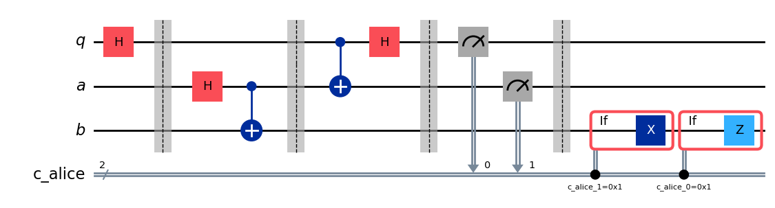
teleport_qc = QuantumCircuit(q, a, b, cr_alice, name='Teleportation')

# Step 1: Prepare message state |+⟩ on q
teleport_qc.h(q[0])
teleport_qc.barrier()

# Step 2: Create entanglement between a and b
teleport_qc.h(a[0])
teleport_qc.cx(a[0], b[0])
teleport_qc.barrier()

# Step 3: Alice's Bell measurement
teleport_qc.cx(q[0], a[0])
teleport_qc.h(q[0])
teleport_qc.barrier()

# Step 4: Alice measures q and a
teleport_qc.measure(q[0], cr_alice[0])
teleport_qc.measure(a[0], cr_alice[1])
teleport_qc.barrier()

# Step 5: Bob's conditional measurements
with teleport_qc.if_test((cr_alice[1], 1)):
    teleport_qc.x(b[0])
with teleport_qc.if_test((cr_alice[0], 1)):
    teleport_qc.z(b[0])

# Draw the circuit
teleport_qc.draw(output='mpl')

לאחר הרצת הפרוטוקול עולה שאלה מרכזית: איך מאמתים שהטלפורטציה עבדה? לא ניתן 'לראות' ישירות את המצב של ה-Qubit של בוב לאחר הפרוטוקול. עם זאת, מכיוון שהכנו את המצב הראשוני $|\psi\rangle$ של אליס (בחרנו $|+\rangle$), אנחנו יכולים להשתמש בסוג מיוחד של סימולציה כדי לבדוק אם ה-Qubit b של בוב הסתיים באותו מצב.

נשתמש ב-AerSimulator עם save_statevector כדי לבדוק אם ה-Qubit b של בוב מסיים במצב הראשוני של אליס ($|+\rangle$). הסימולטור מחשב את וקטור המצב הקוונטי הסופי. ואז מייצג אותו באמצעות plot_bloch_multivector כדי להמחיש את ה-Qubit של בוב (b) בהשוואה למצב הראשוני של אליס (q).

# Simulate the teleportation circuit
sv_simulator = AerSimulator(method='statevector')
teleport_qc_sv = teleport_qc.copy()
teleport_qc_sv.save_statevector()

# Execute the circuit on the statevector simulator
job_sv = sv_simulator.run(teleport_qc_sv)
result_sv = job_sv.result()

# Get the final statevector
final_statevector = result_sv.get_statevector()
print("Visualizing final qubit states:")
display(plot_bloch_multivector(final_statevector))
print("Note that Alice's qubits have collapsed to |00⟩, |01⟩, |10⟩, or |11⟩, while Bob's qubit is in the original state |+⟩.")

Visualizing final qubit states:

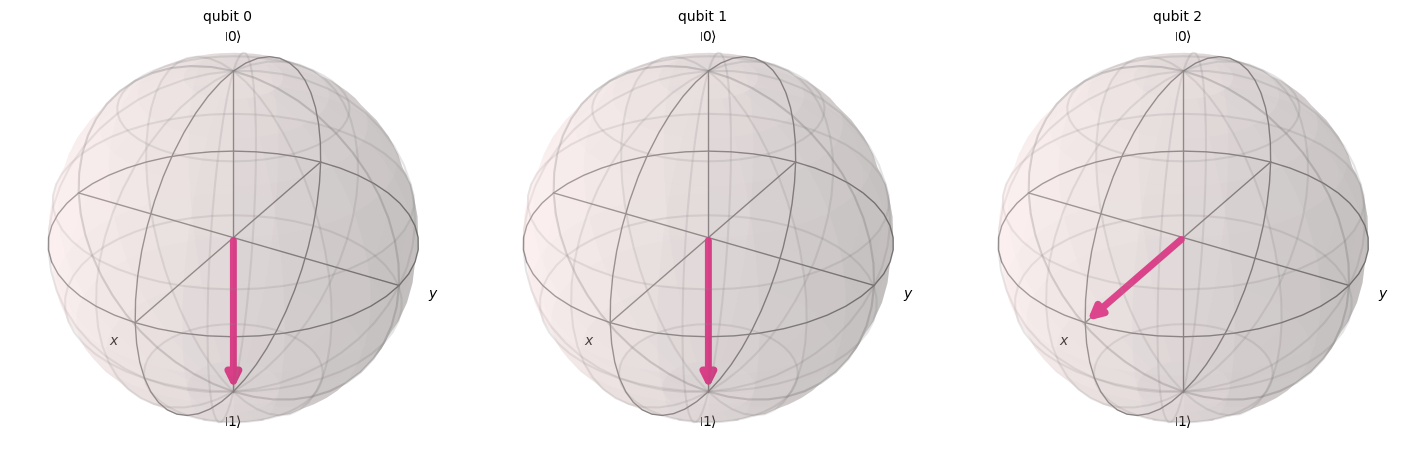
Note that Alice's qubits have collapsed to |00⟩, |01⟩, |10⟩, or |11⟩, while Bob's qubit is in the original state |+⟩.

כפי שאנחנו רואים מהמחשה, שני ה-Qubit הראשונים (השייכים לאליס) התמוטטו ל-0 או 1. בינתיים, ה-Qubit השלישי (השייך לבוב), המיוצג בכדור Bloch השלישי, מצביע לאורך ציר x, מה שמעיד שהוא נמצא במצב $|+\rangle$, כך שיישמנו בהצלחה את פרוטוקול הטלפורטציה הקוונטית!

סיכום

בשלב זה כדאי לעשות סיכום קצר של מה שהשגנו:

• אליס העבירה מצב קוונטי לא ידוע לבוב.
• שום חלקיק פיזי לא הועבר.
• המצב המקורי על ה-Qubit של אליס נהרס, בהתאם למשפט אי-השכפול.